

Plant Count for Field
This analytics automatically detects and counts plants and gaps.
1. Inputs and parameters
- Spectral Index Maps (NDVI by default) *
- Field Boundaries *
- Row vectorization (if not available in input, it will be calculated automatically)
- Theoretical Inter plant spacing *
- Row spacing *
- Deliverables suffix
*Mandatory
Sensor required:
- Multispectral
- RGB
2. Deliverables
- Gaps + suffix.geojson
- Rows with plant count + suffix.geojson
- Plant count + suffix.geojson
- Gaps + suffix.csv
- Rows with plant count + suffix.csv
- Plant count trial + suffix.csv
3. Attributes
The geojson and the corresponding CSV file have the same attributes.
“Gaps” output - only for plants in rows with the following attributes:
- row_index: row id
- gap_id: id of the gap
- gap_length: Length of the gap in meter
“Plant count” output with the following attributes per field:
- gap_length: cumulated gap length in the field in meter
- plant_length: cumulated plant length in the field in meter
- plant_count: number of plants in the field
- row_count: number of rows in the field
“Rows with plant count” output with the following attributes per row:
- row_length: row length in meter
- plant_length: cumulated plant length in the row in meter
- plant_count: number of plants in the row in meter
- gap_length: cumulated gap length in the row in meter
- veg_ratio: plant_length/row_length, between 0 and 1
4. Workflow
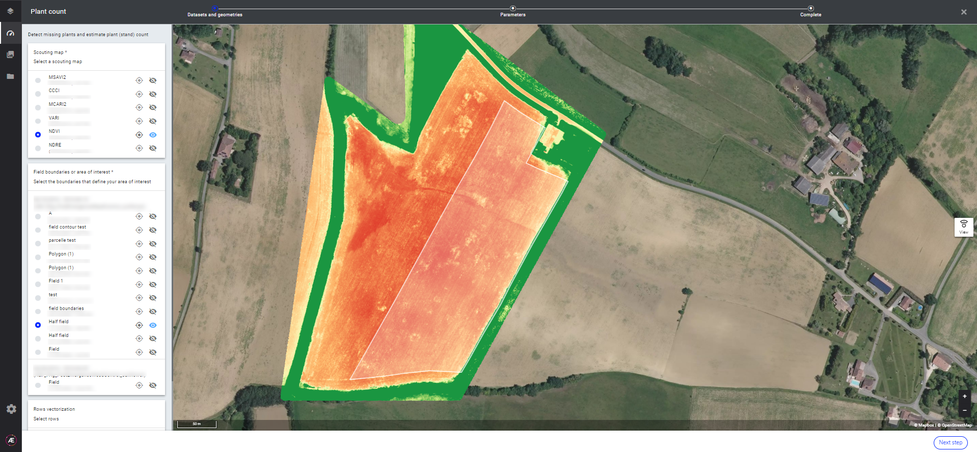
Step 1:
- Select the vegetation indice that will be used to process the Plant and Gap counting (by default: NDVI is selected)
Note: for RGB data sets, select VARI (the VARI indice has to be previously generated) - Select field boundaries*
- Select the rows (optional / if already vectorized)
*field boundaries need to be a vector file. You can obtain this vector by drawing an annotation that represents the field boundaries and converting it into a vector.
Step 2 :
- Fill the inter-plant spacing (distance between 2 plants within the same row)
- Fill in the row spacing (distance between 2 rows)
- Click on Launch
5. How to use it
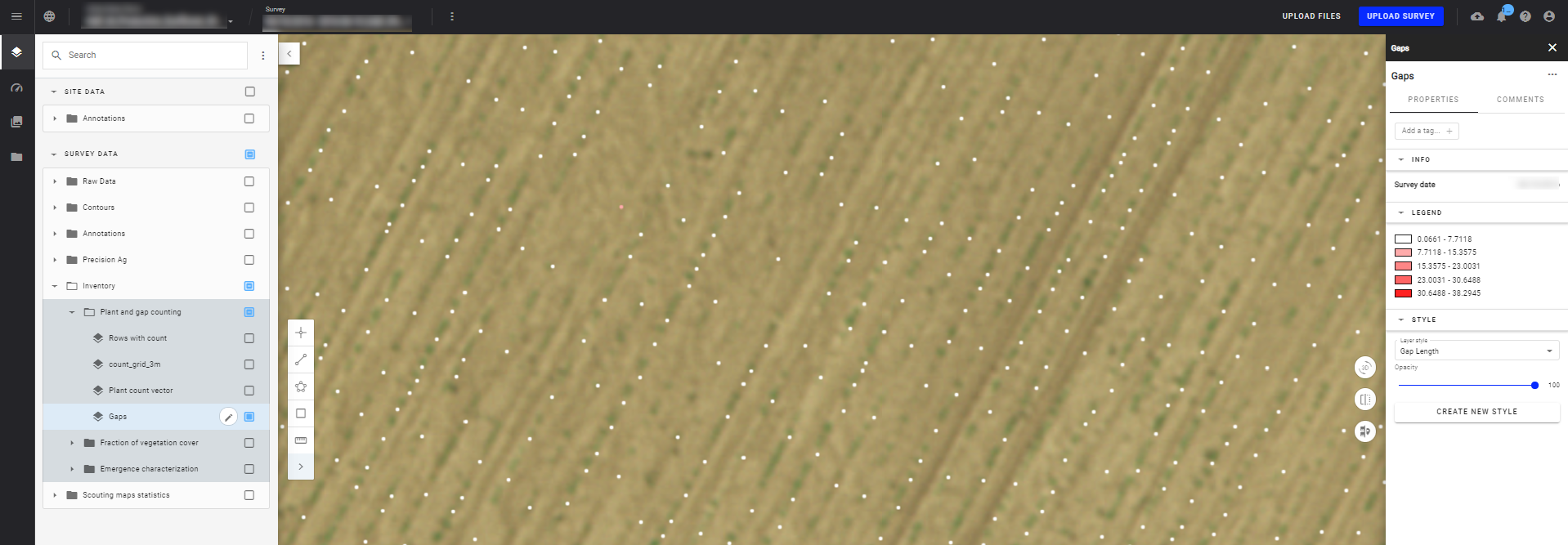
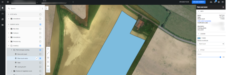
From the layers panel, select the Inventory layer from the SURVEY DATA section and select between plant count or gaps layers to display :
- If you display the Gap layer, it is better to also display the RGB map to locate where is the gaps. Gaps are represented by small dots and depending on the gap length, a specific color is displayed and associated to the legend on the right panel. The gap length can also be displayed if you click on the dot.
- If you display the Plant count layer, the vectorized field will appear. You can click on the field on the map to display its plant number.
Learn more: Vector Layers Styling
