Plant Count & Emergence for Microplot
1. Description
Estimates plant count and emergence for row crops
This article will cover the 3 analytics:
- Plant Count & Emergence from spectral index for microplot
- Plant Count & Emergence from orthomosaic for microplot
- Plant Count & Emergence from reflectance for microplot
2. Prerequisites
Acquisition Prerequisites
The accuracy of the analysis is directly linked to the quality of the input data. To ensure optimal results, please follow these guidelines during image acquisition:
- Bare Soil Requirement: The algorithm is optimized to distinguish vegetation from bare soil.
- Debris and Weeds: If the soil is not "clean" (e.g., significant weed pressure, heavy crop residue, or high moisture levels altering soil color), the algorithm may struggle to correctly identify crop rows and individual plant spacing.
- Growth Stage: Acquisition should ideally take place during the emergence stage, before the crop canopy closes (i.e., before leaves from adjacent plants overlap).
Analysis Prerequisites
| Required | Definition |
| Spectral Index Maps (for Plant Count & Emergence from spectral index for Microplot) |
|
| RGBorthomosaic map (for Plant Count & Emergence from orthomosaic for Microplot) | Raster issue from Photogrammetry or the Generic Scouting Map or Custom Composition Map analytics |
| Reflectance map (for Plant Count & Emergence from reflectance for Microplot) | Raster map issue from Photogrammetry or imported in Aether |
| Inter-plants spacing | Theoretical interplant spacing (within the row) It is mandatory to see the bare ground between two plants on the map |
| Microplots vector | Vector file containing microplot boundaries |
| Optional | Definition |
| Row vectorization | Vector file containing the digitized rows (if already available). |
| Deliverables suffix | A suffix applied to all deliverable names |
3. Workflow
3.1 Plant Count & Emergence from spectral index for microplot
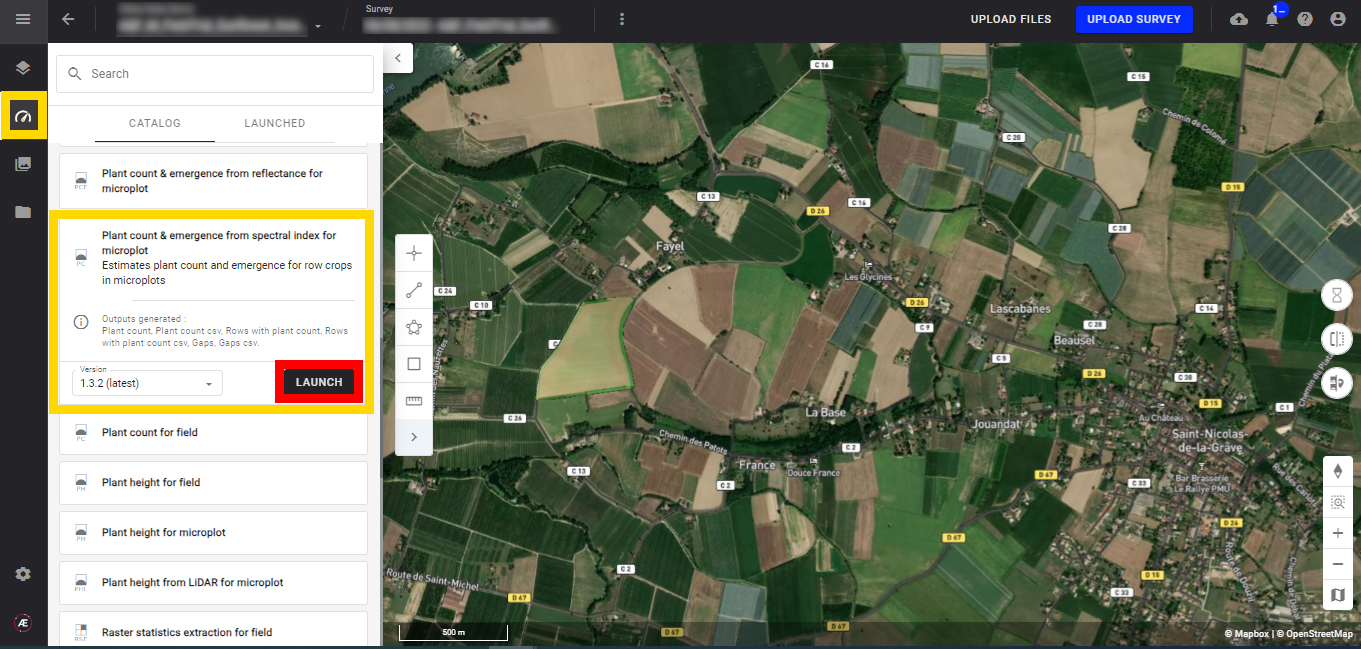
Step 1 - In the "Analytics" tab, search and select "Plant Count & Emergence from spectral index for microplot" and click on "LAUNCH".
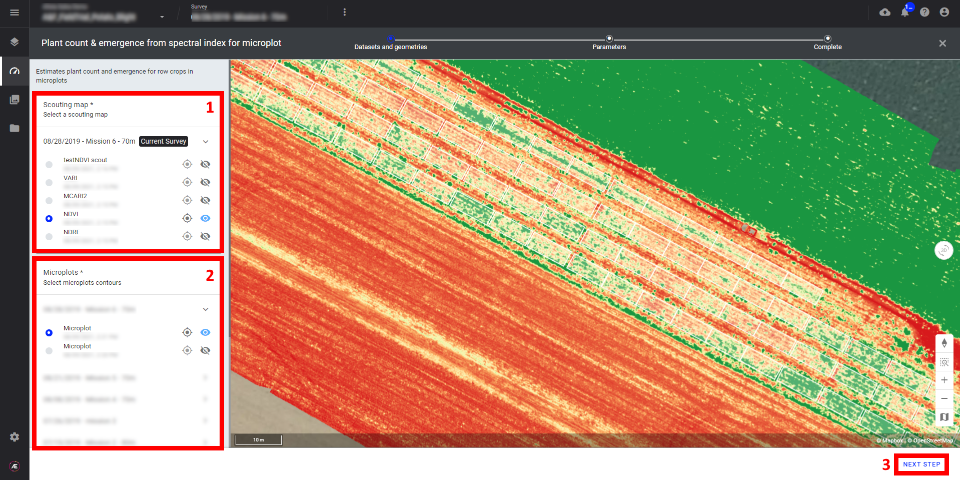
Step 2 - Select the "Scouting Map" (spectral index map) (1) and the "field boundaries" (microplot file) (2) and click on "NEXT STEP" (3).
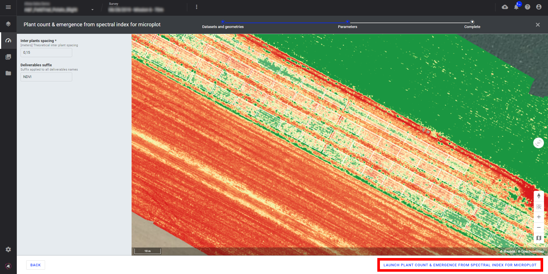
Step 3 - Fill in the "Inter plants spacing" (the unit is in meters) and "Deliverables suffix",
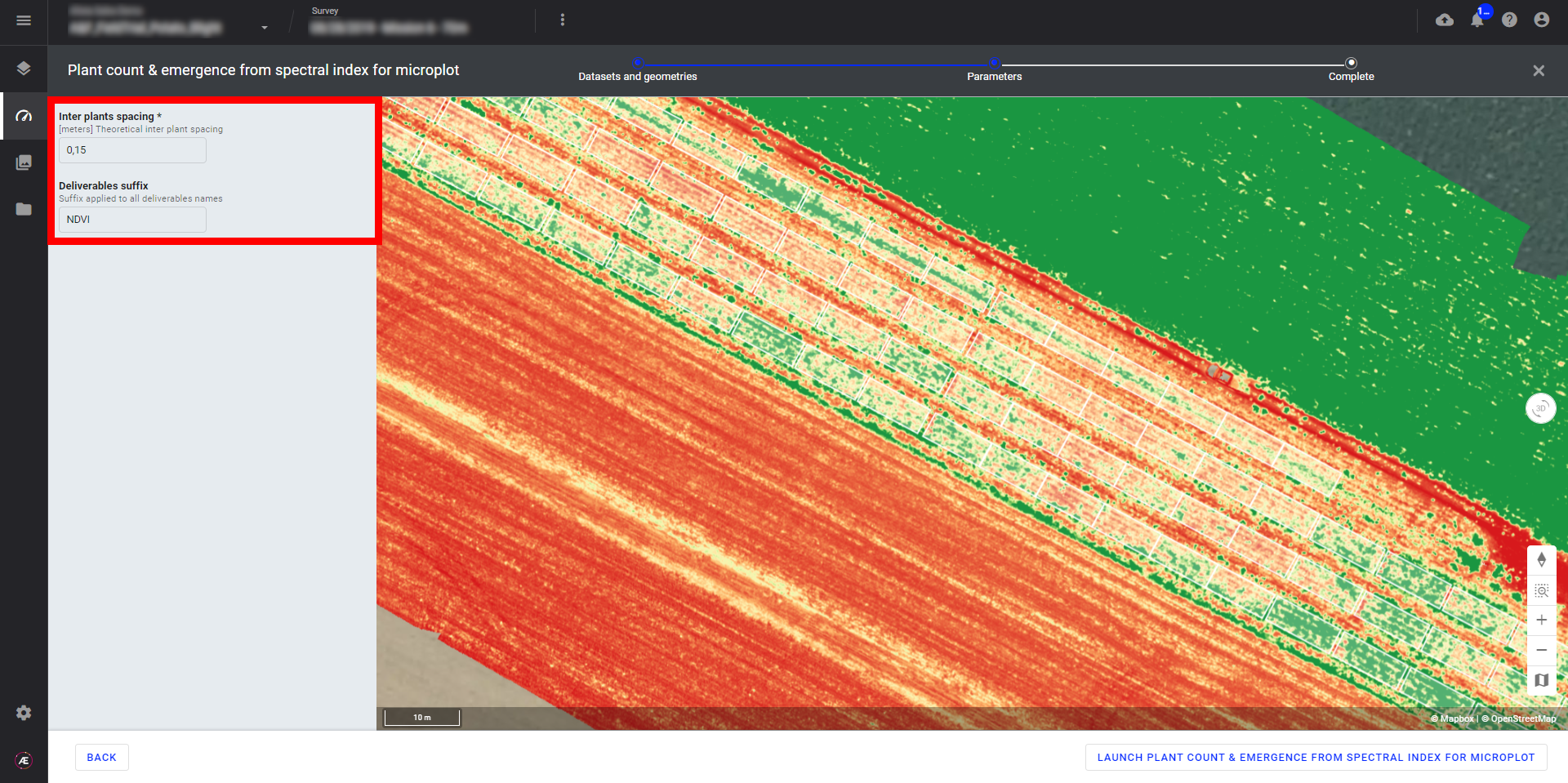
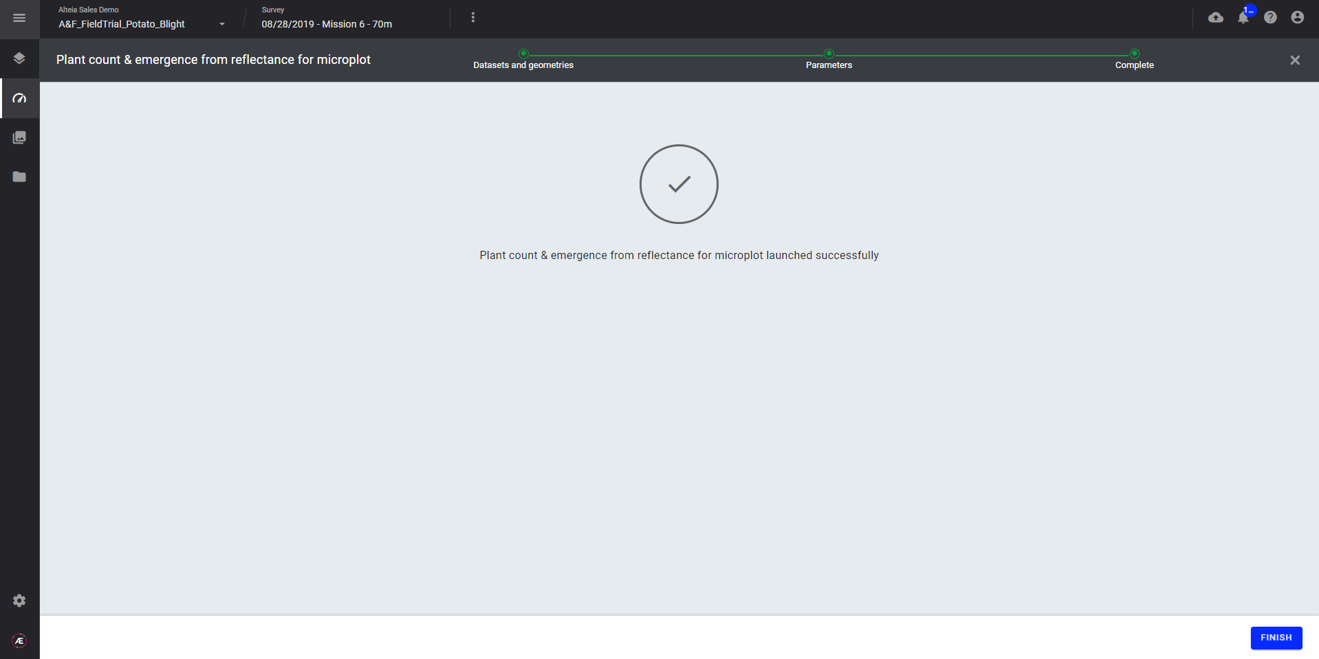
Step 4 - Click on "LAUNCH PLANT COUNT & EMERGENCE FROM SPECTRAL INDEX FOR MICROPLOT".
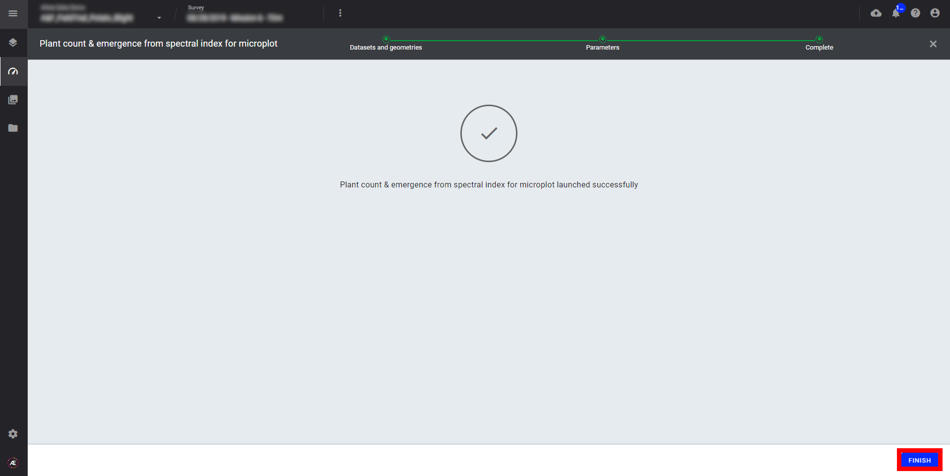
Step 5 - Click on "FINISH" to leave the analytics.
3.2 Plant Count & Emergence from orthomosaic for microplot
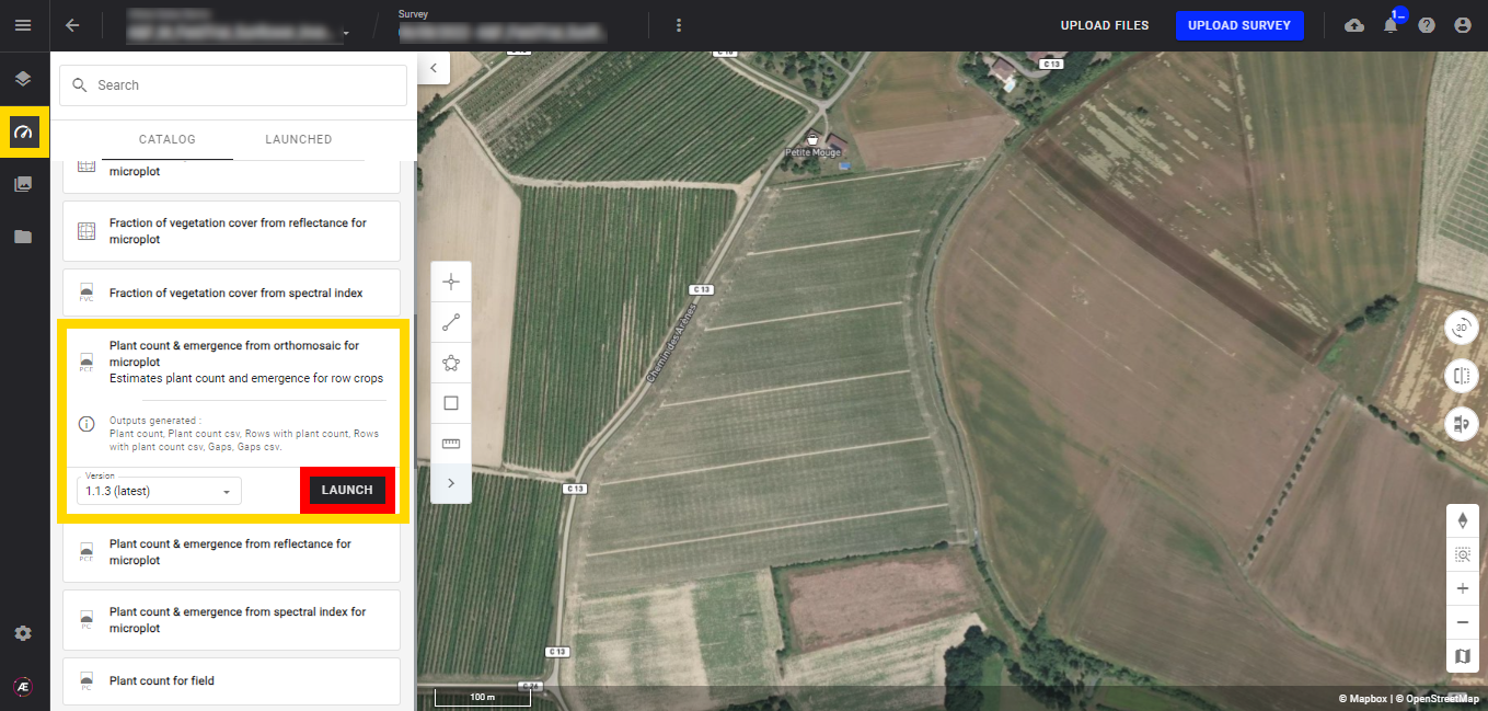
Step 1 - In the "Analytics" tab, search and select "Plant Count & Emergence from orthomosaic for microplot" and click on "LAUNCH".
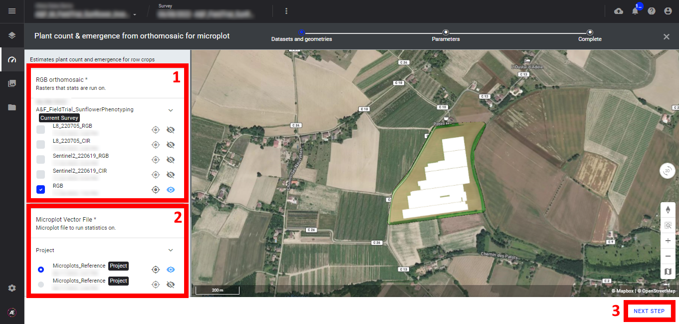
Step 2 - Select the "RGB orthomosaic" map (1) and the "Microplot Vector File" (2) and click on "NEXT STEP" (3).
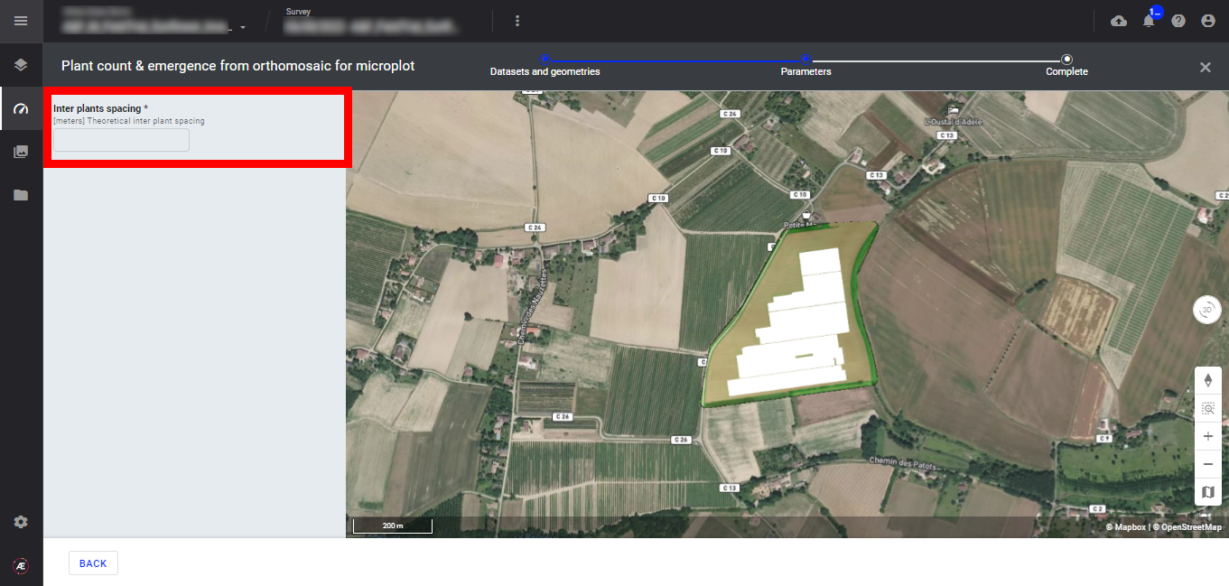
Step 3 - Fill in the "Inter plants spacing", the unit is in meters.
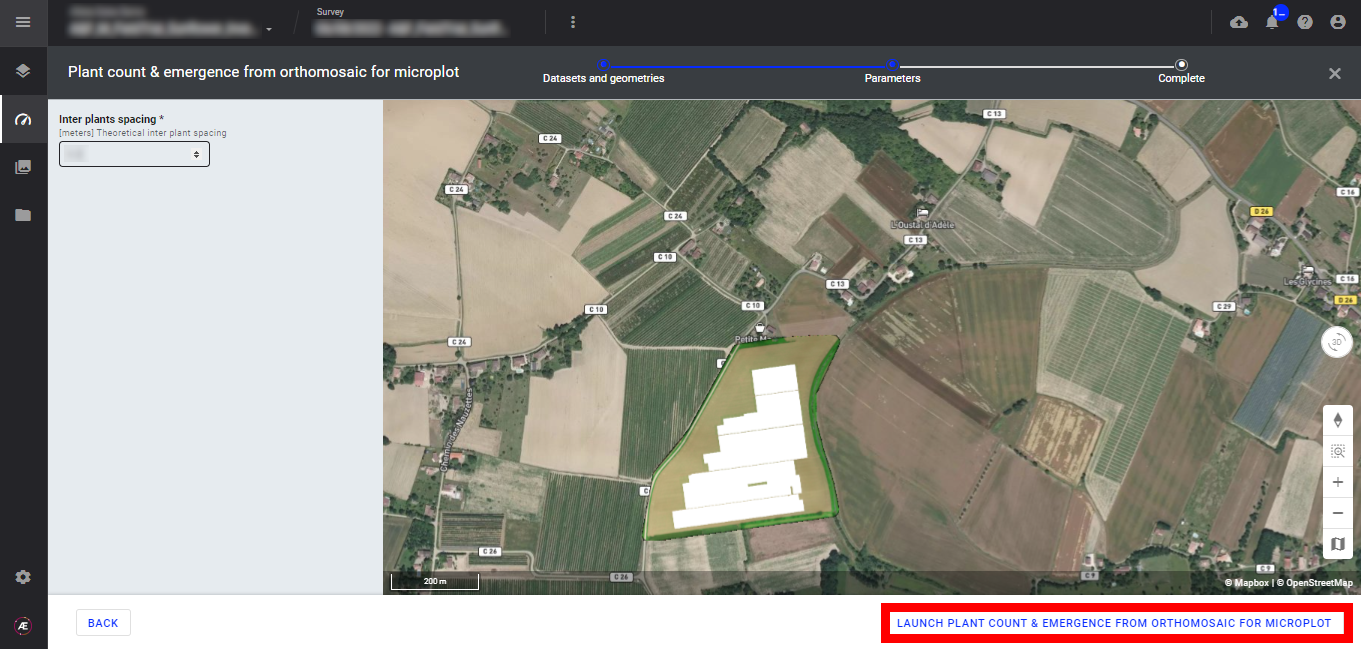
Step 4 - Click on "LAUNCH PLANT COUNT & EMERGENCE FROM ORTHOMOSAIC FOR MICROPLOT".
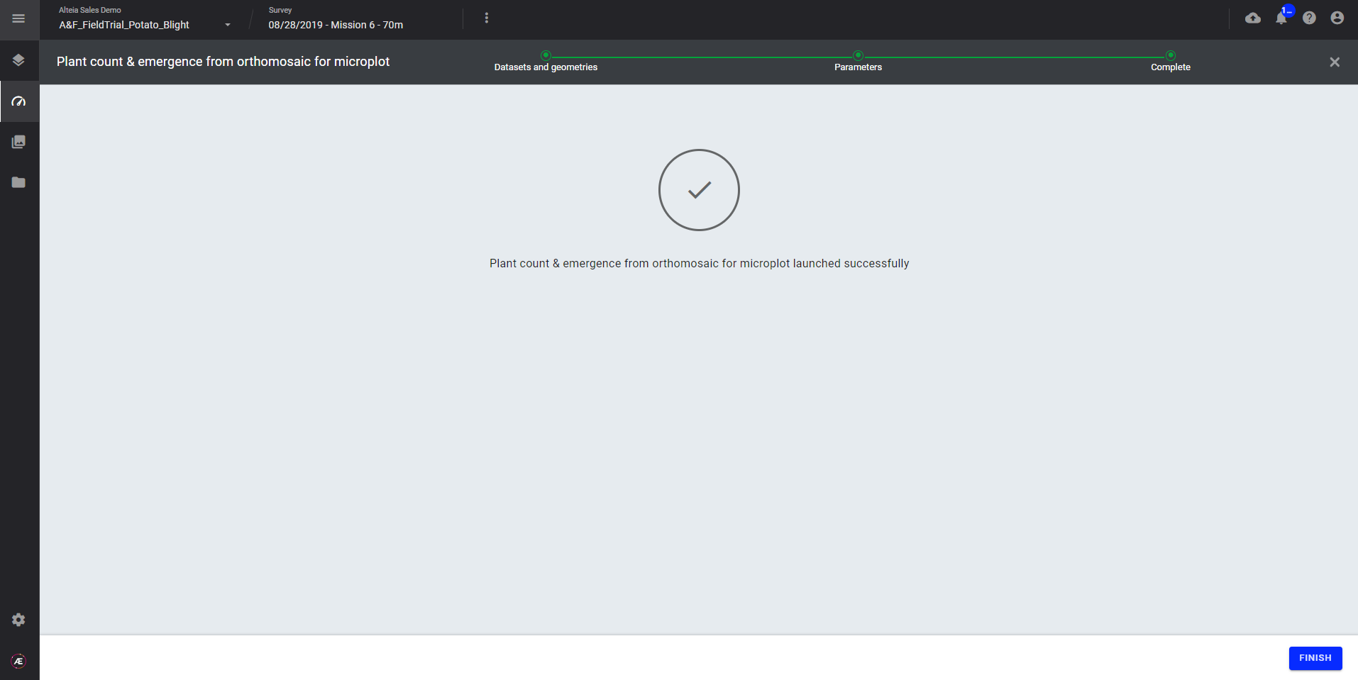
Step 5 - Click on "FINISH" to leave the analytics.
3.3 Plant Count & Emergence from reflectance for microplot
Step 1 - In the "Analytics" tab, search and select "Plant Count & Emergence from reflectance for microplot" and click on "LAUNCH".

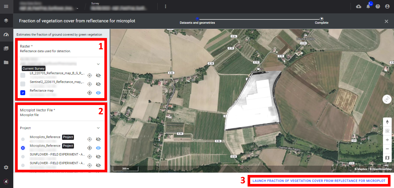
Step 2 - Select the "Raster" (reflectance map) (1) and the "microplot vector file" (2) and click on "LAUNCH PLANT COUNT & EMERGENCE FROM REFLECTANCE FOR MICROPLOT" (3).
Step 3 - Click on "FINISH" to leave the analytics.
4. Status and Progression
Check in the "LAUNCHED" tab that the analytics is in progress.
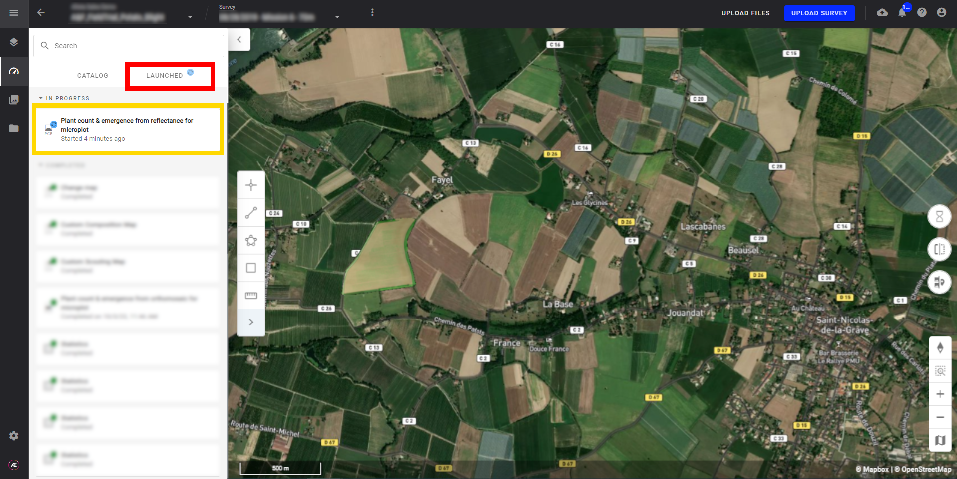
Aether will notify the user that the analytics results are available.
5. Results
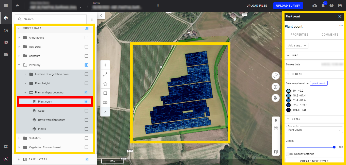
5.1 Layers
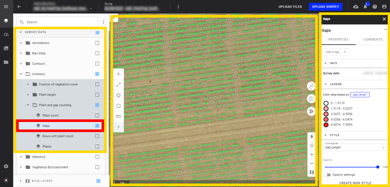
In the "Inventory" subgroup of "SURVEY DATA" a new subgroup "Plant and gap counting" is created with 4 layers:
- Plant count
Display the plant count layer, and the microplots appear. The microplots will also be colored depending on the selected attribute and its corresponding values.
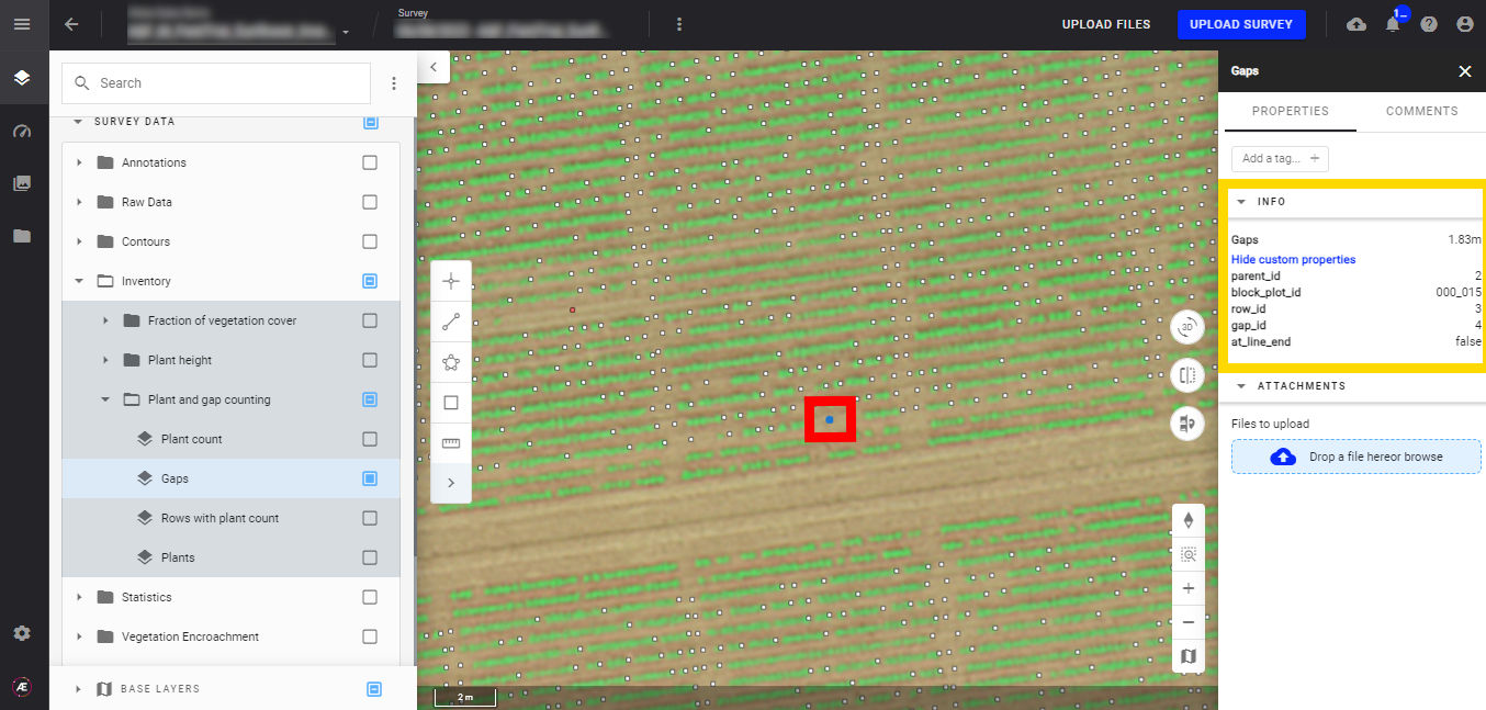
- Gaps
You can also display the RGB map to identify where the gaps are located. Gaps are represented by small dots, and their color depends on the gap length. Refer to the "Legend" for color/distance definitions.
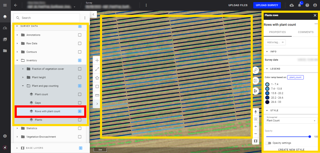
- Rows with plant count
6. Deliverables
6.1 Files
In the "Download" section find files issue from the analytics.
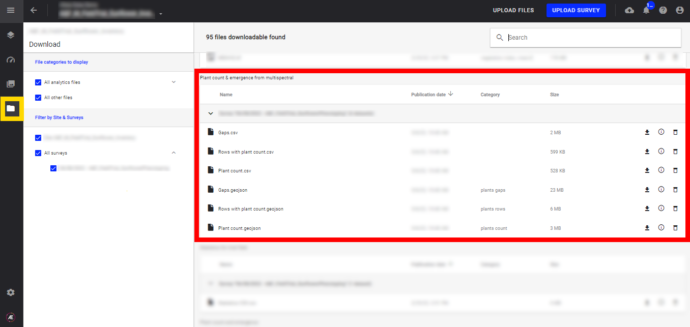
Once the analytics is run, the deliverables can be exported in two standard formats, vector format such as "geoJSON," and "CSV".
6.2 Attributes
List of attributes for each format:
| Deliverable | File Format | Attributes |
|---|---|---|
| Gaps | geoJSON |
|
| Rows with plant count | geoJSON |
|
| Plant count | geoJSON |
|
7. Optimization Tips
While the algorithm delivers accurate results in the majority of cases, its performance depends heavily on data consistency and spatial uniformity. To ensure optimal processing, keep the following configurations in mind:
- Vector Homogeneity: Ensure that your microplot vectors (the boundaries) are drawn as uniformly as possible. Significant variations in size, orientation, or distance between plots within the same trial can hinder the algorithm's ability to cross-reference and align the plots effectively.
Troubleshooting anomalies: If you notice errors in a specific area, first check the soil cleanliness and the geometric regularity of your microplot vectors in that zone.
8. Quality check the results
This section allows identify potential anomalies on your trial plots.
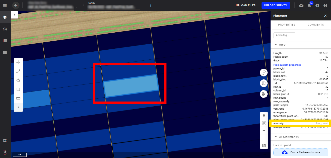
8.1 Check the "anomaly" attribute
In a plant count vector output, click on a plot to see if there is an anomaly for that given plot. Or extract the CSV file to see a report of the anomalies for all plots.
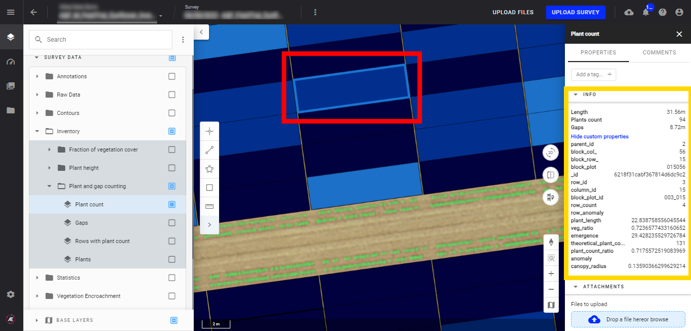
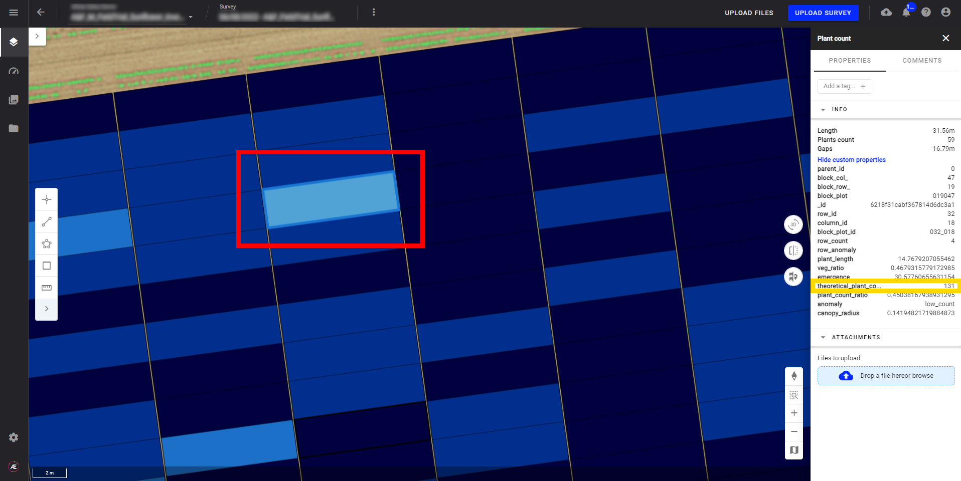
8.2 Check the "theoretical_plant_count" attribute
In the plant count vector output, if the values are very different from your theoretical plant count, there is probably an anomaly.
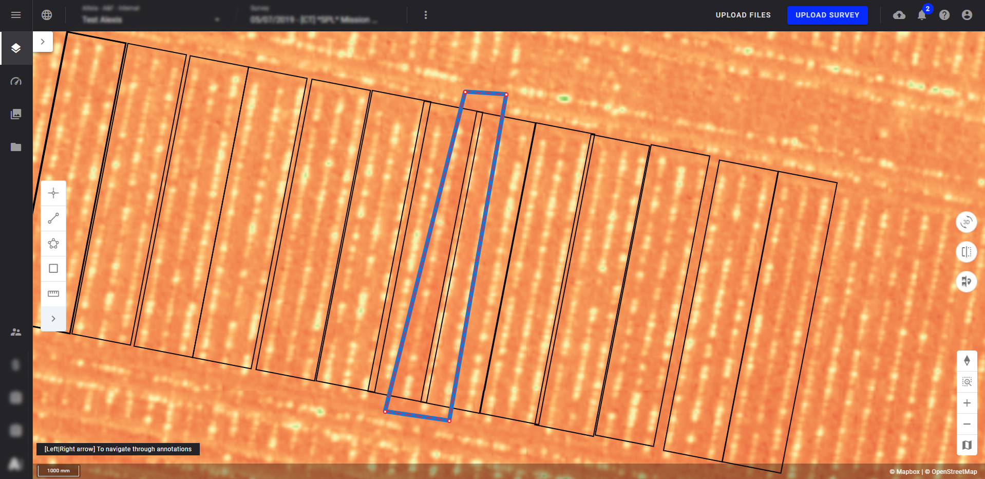
8.3 Check the microplot coregistration
If the plot contour isn't well located around the plants, the results can be impacted. Use a scouting map (like NDVI) in the background to better identify the plant rows and make corrective actions.
The example below shows an overlay of microplots on a plant row. The plants present in this row are therefore difficult to count, which affects the results delivered.